• Formulas
  • Excel Tips & Tricks
  • Excel Charting
  • Tutorials
  • VBA
  • Book Store
  • More  
    • Blog
    • Download Area
    • Excel Video Tutorials
You are here: Home / Excel Charting / Break Your Pivot Table Filters Into Multiple Columns

Break Your Pivot Table Filters Into Multiple Columns

November 2, 2013 by Barbara

Before I found out about this little tip, the multiple stacked report filters in my Pivot Tables REALLY annoyed me. So, here is how to avoid all of those stacked up messy filters. Yuk.

I have used in my example below a standard Pivot Table with filters of Sales Person, Customer and Customer Type. Usually all of the filters are stacked on top of each other just like this..

blue down arrwo

Pivot Table Filters


Let’s make it look a lot better!…well I think it looks a lot better when you have done this…….

  • Right click anywhere inside the Pivot Table.
  • Select Pivot Table Options.
  • In Options Dialog Box- Layout and Format go to the setting- ‘Report filters fields per column’
  • Change this setting to how many filter fields you want in each column. In my example I am choosing 1 per column to give a neater and more easily navigable Pivot Table.


Pivot Table Filters1


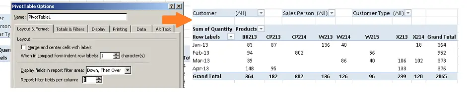
So….how much better does that Pivot Table look..what do you think?


Want to watch the Video Excel Tip?

More Excel Tips


1. Default your Pivot Tables to SUM not COUNT

2. Why you NEED to know how to build Dashboards in Excel

3. Find and replace line breaks in Excel

Advanced Excel & Power Pivot Training Classes

Become a Data Analysis & Dashboarding Monster!

power-pivot-excel-school-introduction-and-benefits-v4


Filed Under: Excel Charting, Excel Tips& Tricks, Pivot Tables Tagged With: Excel, Excel Tips, formatting

Comments

  1. Gaurav Kumar says

    February 5, 2014 at 7:16 am

    very nice tip, i never got into to much depth of pivot so was not aware of this thing also.

    it gives a pretty look to pivots especially with lots of columns in it.

    thanks for very simple & nice tip

Trackbacks

  1. Formula Friday - How To Calculate The Number Of Workdays Between Two Dates Using NETWORKDAYS says:
    May 15, 2015 at 8:13 pm

    […] Break Your Pivot Table Filters Into Multiple Columns […]

  2. Formula Friday- COUNTIFS With Multiple Criteria In Excel says:
    May 22, 2015 at 8:58 pm

    […] Break Your Pivot Table Filters Into Multiple Columns […]

SHARE

Tweet

Additional Info

Need Answers To Excel Questions Like These?

*How Do I Create A Timestamp In Excel?
*I Want To Change The Width Of The bars On My Excel Chart
*How Can I Find Out The Length Of My Text in Excel? Click the link below to receive more Excel tips' and my Free Ebook

Sign Up For My FREE Excel Tips Newsletter and receive your own E-book of my Top 50 Excel Tips.

New To Excel? This Is A Great Place To Start!!

excel-formulas-ad-5 Excel Basics
Scrollbars
Colour of Sheet Tabs
Conditional Formatting
Calculations Introduction

Advanced Excel

Power BI Webinar Excel Expert Course Excel Dashboard Course
Data Validation Lists
Create A Timestamp
Create Table Of Contents

Excel Charting

Self Expanding Charts
One Click Charts
Create Quick Dynamic Charts
Easy Combination Charts

Video Tutorials-If You Like To Learn By Watching

Subscribe to YouTube to get notified of of new Excel videos.


Self Expanding Chart
Delete Obsolete Items From A Pivot Table-Excel 2007
What Are Pivot Tables- Create Your First One
Enable The DeveloperTab In Excel

Some Fun Stuff

Pivot Table Song

Tags

Blog Cells Excel Excel Charting Excel Formulas excel tip Excel Tip Category Excel Tips Excel Tips& Tricks excel tutorials Excel Videos Excel Video Tutorials formatting Formula formula friday Formulas macro Macro Mondays Macros Pivot Tables Power BI Power Query Tutorials vb VBA Worksheets

Recommended Excel Resources

Free Excel Dashboard Webinar

Copyright © 2019 · Enterprise Pro Theme on Genesis Framework · WordPress · Log in

privacy policy